What is control theory and why do we need it?

Control is ubiquitous—from humanoid robots and reusable launch vehicles to financial systems, control is essential: specifically, control is needed wherever we want a manufactured object to operate autonomously and achieve its objectives. People from different backgrounds develop their own control algorithms to accomplish missions autonomously. The field that represents abstract systems using differential or difference equations and studies their behavior under designed control algorithms is called control theory. We will go through a high-school physics case to design your first control algorithm in the following.

A high-school physics case: an object on an inclined plane

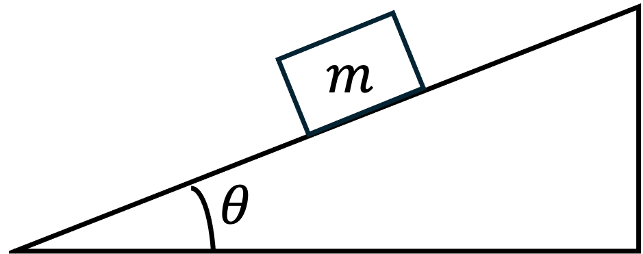
Warm-up Question

Given the frictionless block and inclined plane shown above, the plane makes an angle $\theta$ with the horizontal. The block has mass $m$, and the gravitational acceleration is $g$. The block is initially at rest at a point a distance $l$ up the slope from the bottom.

Question: After it is released at $t=0$, how long does it take for the block to reach the bottom of the incline?

Answer

Applying Newton's second law along the inclined plane:
From the force analysis, the gravitational force component acting on the block along the plane is $mg \sin\theta$, thus the acceleration along the inclined plane is $a = g \sin\theta$. Using the kinematic equation $l = v_0t+ \frac{1}{2} a t^2$ with initial velocity $v_0=0$, the time required for the block to travel a distance $l$ along the inclined plane is $t = \sqrt{\frac{2l}{g \sin\theta}}$.

The warm-up question above is a simple case in high-school physics. Now you have a scenario that the system, frictionless block, moves without any human intervention.

A step further:

Next, consider that you want to apply "control": you wish to change the destination of the block to the top of the inclined plane, position $2l$. How can you design the force applied to the block?

Answer:

We define the upward direction along the inclined plane as the positive direction; therefore, the displacement we need to achieve is $2l - l = l$. The net acceleration along the inclined plane in the upward direction is $a_x - g\sin\theta$, where $a_x$ is the designed acceleration (by Newton's second law, the control force is $F = ma_x$). Using the kinematic equation with zero initial velocity:

$$x = \frac{1}{2} a T^2,$$

we obtain

$$l = \frac{1}{2}(a_x - g\sin\theta)T^2.$$

After rearranging, we obtain the relationship between the mission duration $T$ and the designed acceleration $a_x$:

$$a_x = \frac{2l}{T^2} + g\sin\theta. \tag{1}$$

Well done! You've used high school physics tools to design your first open-loop control algorithm: the block driven by the designed acceleration $a_x$ can reach the goal position in the predefined mission duration $T$, as long as $a_x > g\sin\theta$.

Reflection

Where do these equations come from?

We were taught to use equations like $v= v_0+at$ and $x = v_0t+\frac{1}{2}at^2$ to solve problems in high school. But where do these kinematic equations come from?

Some classmates in high school already knew that acceleration $a$ is the derivative of velocity $v$, and velocity is the derivative of position $x$, and they are all functions of time $t$. Instead of treating the acceleration $a$ as a constant, we generalize it:

$$\dot x(t) = v(t)\\ \dot v(t) = a(t),$$

where these above are exactly the simple case of ordinary differential equation (ODE). Solving the ODEs above gives you the general form (Now we need mathematical knowledge back to undergrad):

Solving the velocity equation

The velocity dynamics are given by

$$\dot v(t) = a(t).$$

Integrating both sides from $0$ to $t$, we obtain

$$v(t) = v(0) + \int_0^t a(\tau)\, d\tau.$$

Solving the position equation

The position dynamics are

$$\dot x(t) = v(t).$$

Substituting the expression of $v(t)$ yields

$$x(t) = x(0) + \int_0^t v(\tau)\, d\tau= x(0) + \int_0^t \left( v(0) + \int_0^\tau a(s)\, ds \right) d\tau.$$

Separating the terms, we obtain

$$x(t)= x(0) + v(0)t + \int_0^t \int_0^\tau a(s)\, ds\, d\tau.$$

Exchanging the order of integration

By changing the order of integration, we have

$$\int_0^t \int_0^\tau a(s)\, ds\, d\tau= \int_0^t (t-s)\, a(s)\, ds.$$

Plug the result above back, we have the solution for velocity and position:

$$v(t) = v(0) + \int_0^t a(s)\, ds, \\ x(t) = x(0) + v(0)\, t + \int_0^t (t - s)\, a(s)\, ds .$$

Treating the acceleration as a constant, $a(t) = a$, set the initial position as $x(0)=0$, and solve the integration, we recover the equation back to high school:

$$v(t) = v(0) + at, \\ x(t) = v(0)\, t + \frac{1}{2}at^2 .$$

So far, we understand that the educator alleviate the burden for high school student by directly telling the analytic solution of the ODEs. The case above is already the most simple case. In the harsh reality, we need to solve the ODE to have a control law. What should we do with the more complex system? Is there anyway to escape the burdensome computation?

Besides, in the above design, we'd better hope there is nothing happened during the whole process: once the control law is encoded, it never cares about the information happening in the mission. However, a lot of exception can happen like the slight movement of the inclined plane. In this case, we wish the control can adjust according to the real-time situation.

Two terms to sum up the problems above is design complexity and adaptability.

Can we design a control law without solving the ODE?

Luckily, the predecesor in control provides the lazy way to design a feedback control law: intuitively, achieving a goal position and velocity (which is 0) means exerting influence on position $x$ and velocity $v$. For example, the current position is $1$, and we wish it to be $0$, so it would be great if we can drive it approaches that. However, we cannot directly pick up the block and place it to the goal position (Remember, you can only push it along the inclined plane).

Some of people learns the concept of negative feedback regulation back to high school biology: the punishment comes when the object goes away from its goal to correct it. It seems a good mechanism we can apply to the block: the punishment (horizontal force) comes and drives it to its goal position when it is far away from its goal. How can we design it in a mathematical way?

It turns out that the feedback control form is simple:

$$a(t) = -k_1x(t)-k_2v(t)$$

Plugging this form back to the ODEs, $\dot x(t) = v(t)$ and $\dot v(t)=a(t)$, we have

$$\dot{x}(t)=v(t) \\ \dot{v}(t)=-k_1 x(t)-k_2 v(t)$$

For the system with state feedback control law $a(t) = -k_1 x(t) - k_2 v(t)$, the resulting closed-loop dynamics can be written as the second-order linear ODE

$$\ddot x(t) + k_2 \dot x(t) + k_1 x(t) = 0, \tag{1}$$

whose characteristic equation is given by $\lambda^2 + k_2 \lambda + k_1 = 0$. The block can achieve the goal (or it is asymptotically stable in a rigorious term) if and only if all eigenvalues of this polynomial have strictly negative real parts, which is guaranteed by the simple algebraic conditions $k_1 > 0$ and $k_2 > 0$, without the need to explicitly solve the ODE for $x(t)$.

Verification

Recall that the block dynamics along the inclined plane are

$$\dot x(t) = v(t), \qquad \dot v(t) = a(t) - g\sin\theta .$$

To move the block to the top of the incline at position $x = 2l$, we define the position error

$$e(t) := x(t) - 2l .$$

Driving the block to the goal position means enforcing

$$e(t) \to 0, \qquad \dot e(t) = v(t) \to 0 .$$

Choosing a feedback control law

We choose the following feedback acceleration:

$$a(t) = g\sin\theta - k_1 e(t) - k_2 v(t),$$

where $k_1 > 0$ and $k_2 > 0$ are design parameters.

Substituting this control law into the dynamics gives

$$\dot e(t) = v(t),\\ \dot v(t) = -k_1 e(t) - k_2 v(t).$$

Equivalently, the error dynamics satisfy the second-order linear ODE

$$\ddot e(t) + k_2 \dot e(t) + k_1 e(t) = 0. \tag{2}$$

Choosing concrete numbers

Now we choose explicit numerical values for the feedback gains. Let

$$k_1 = 4, \qquad k_2 = 4.$$

Then equation (2) becomes

$$\ddot e(t) + 4 \dot e(t) + 4 e(t) = 0,$$

whose characteristic equation is

$$\lambda^2 + 4\lambda + 4 = (\lambda + 2)^2 = 0.$$

Both eigenvalues are $\lambda = -2$, which has a strictly negative real part. Therefore,

$$e(t) \to 0, \qquad \dot e(t) \to 0 \quad \text{as } t \to \infty.$$

Interpretation for the block

Starting from the initial condition $x(0) = l$ and $v(0) = 0$, the position error $x(t) - 2l$ converges to zero, the velocity converges to zero, and the block comes to rest exactly at the top of the inclined plane.

The explicit control input applied to the block is

$$\boxed{ a(t) = g\sin\theta - 4\bigl(x(t) - 2l\bigr) - 4v(t) }$$

This simple numerical choice verifies that the feedback control law drives the block to the desired position without explicitly solving the system trajectories.

Matching the initial acceleration

We can connect the feedback control law to the original open-loop control form from equation (1), $a_x = \frac{2l}{T^2} + g\sin\theta$.

From the feedback control law,

$$a(t) = g\sin\theta - k_1\bigl(x(t)-2l\bigr) - k_2 v(t),$$

the initial acceleration is given by

$$a(0) = g\sin\theta - k_1\bigl(x(0)-2l\bigr) - k_2 v(0).$$

Using the initial conditions $x(0)=l$ and $v(0)=0$, we obtain

$$a(0) = g\sin\theta + k_1 l.$$

If we wish this initial acceleration to match the open-loop acceleration designed earlier,

$$a_x = \frac{2l}{T^2} + g\sin\theta,$$

we can choose

$$\boxed{ k_1 = \frac{2}{T^2}. }$$

This choice ensures that the feedback control law produces the same acceleration as the open-loop design at the initial time $t=0$.

Conclusion

Congratulations! You've just designed your first control algorithms—both open-loop and closed-loop—using nothing more than high school physics and a bit of calculus.

Key takeaways:

1. Open-loop control designs a fixed input trajectory based on initial conditions, but cannot adapt to disturbances
2. Closed-loop (feedback) control continuously measures the system state and adjusts the input, providing robustness and adaptability
3. Avoiding ODE solutions: Feedback control allows us to design controllers without explicitly solving differential equations—we only need to check algebraic stability conditions
4. The power of linearity: For linear systems, stability analysis reduces to checking eigenvalues of characteristic polynomials

This simple inclined plane example contains the fundamental ideas that scale to complex robots, aircraft, and autonomous vehicles. In future tutorials, we'll explore:

• Nonlinear systems and Lyapunov stability
• Optimal control and the Linear Quadratic Regulator (LQR)
• Safety-critical control with Model Predictive Control (MPC) and Control Barrier Functions (CBFs)

Further Reading

• Youtube Channel
• Podcast

---

Posted on Feb 5, 2026